Language Details¶

The following is a fairly extensive introduction to the grama language. This is (admittedly) not a great place to start learning how to use py_grama, but is instead provided as a reference.

grama is a conceptual language, and py_grama is a code implementation of that concept. This page is a description of both the concept and its implementation.

Running example¶

We’ll use a running example throughout this page; the built-in py_grama Cantilever Beam model.

import grama as gr
from grama.models import make_cantilever_beam

md_beam = make_cantilever_beam()
md_beam.printpretty()

model: Cantilever Beam

  inputs:
    var_det:
      w: [2, 4]
      t: [2, 4]
    var_rand:
      H: (+1) norm, {'loc': 500.0, 'scale': 100.0}
      V: (+1) norm, {'loc': 1000.0, 'scale': 100.0}
      E: (+0) norm, {'loc': 29000000.0, 'scale': 1450000.0}
      Y: (-1) norm, {'loc': 40000.0, 'scale': 2000.0}
  functions:
    cross-sectional area: ['w', 't'] -> ['c_area']
    limit state: stress: ['w', 't', 'H', 'V', 'E', 'Y'] -> ['g_stress']
    limit state: displacement: ['w', 't', 'H', 'V', 'E', 'Y'] -> ['g_disp']

Objects¶

grama focuses on two categories of objects:

data (df): observations on various quantities, implemented by the Python package Pandas
models (md): functions and a complete description of their inputs, implemented by py_grama

For readability, we suggest using prefixes df_ and md_ when naming DataFrames and models.

Data¶

Data are observations on some quantities. Data often come from the real world, but data are also used to inform models, and models can be used to generate new data. py_grama uses the Pandas DataFrame implementation to represent data. Since data operations are already well-handled by Pandas, py_grama uses the existing Pandas infrastructure and focuses on providing tools to handle models and their interface with data.

Models¶

Models in grama have both functions and inputs. py_grama implements models in the Model class, which in turn have three primary objects:

Domain: Defines bounds on variables
Density: Defines a joint density for variables
List ofFunctions: Maps variables to outputs

Domain¶

The domain of the model defines bounds for all the variables. If a variable is not included in the domain object, it is assumed to be unbounded. The model above has bounds on t, w, both of which are [2, 4].

Density¶

The density of the model defines a joint density for the random variables. If a variable is included in the density it is random, otherwise it is deterministic. The model above has a joint density on H, V, E, Y. The model summary gives details on each marginal distribution.

Functions¶

A function has a set of variables, which map to a set of outputs; for instance, the cross-sectional area function above maps ['w', 't'] -> ['c_area']. The other functions take more variables, all of which map to their respective outputs.

Inputs¶

The full set of model inputs are organized into:

	Deterministic	Random
Variables	`md.var_det`	`md.var_rand`
Parameters	`md.density.marginals[var].d_param`	(Future*)

Variables are inputs to the model’s functions
- Deterministic variables are chosen by the user; the model above has w, t
- Random variables are not controlled; the model above has H, V, E, Y
Parameters are inputs to the model’s density
- Deterministic parameters are currently implemented; these are listed under var_rand with their associated random variable
- Random parameters* are not yet implemented

The full set of variables is determined by the domain, density, and functions. Formally, the full set of variables is given (in pseudocode) by domain.var + [f.var for f in functions]. The set of random variables is then given by domain.var + [f.var for f in functions] - density.marginals.keys(), while the deterministic variables are the remainder var_det = var_full - var_rand.

Verbs¶

Verbs are used to take action on different grama objects. We use verbs to generate data from models, build new models from data, and ultimately make sense of the two.

The following table summarizes the categories of py_grama verbs. Verbs take either data (df) or a model (md), and may return either object type. The prefix of a verb immediately tells one both the input and output types. The short prefix is used to denote the pipe-enabled version of a verb.

Verb Type	Prefix (Short)	In	Out
Evaluate	`eval_` (`ev_`)	`md`	`df`
Fit	`fit_` (`ft_`)	`df`	`md`
Transform	`tran_` (`tf_`)	`df`	`df`
Compose	`comp_` (`cp_`)	`md`	`md`
Plot	`plot_` (`pt_`)	`df`	(Plot)

Since py_grama is focused on models, the majority of functions lie in the Evaluate, Fit, and Compose categories, with only a few original Transform utilities provided. Some shortcut plotting utilities are also provided for covenience.

py_grama verbs are used to both build and analyze models.

Model Building¶

The recommended way to build py_grama models is with composition calls. Calling Model() creates an “empty” model, to which one can add.

md = gr.Model()
md.printpretty()

model: None

  inputs:
    var_det:
    var_rand:
  functions:

We can then use Compose functions to build up a complete model step-by step. We recommend starting with the functions, as those highlight the required variables.

md = gr.Model("Test") >> \
     gr.cp_function(
         fun=lambda x: [x[0], x[1]],
         var=["x0", "x1"],
         out=2,
         name="Identity"
     )
md.printpretty()

model: Test

  inputs:
    var_det:
      x0: (unbounded)
      x1: (unbounded)
    var_rand:
  functions:
    Identity: ['x0', 'x1'] -> ['y0', 'y1']

Note that by default all of the variables are assumed to be deterministic. We can override this by adding marginal distributions for one or more of the variables.

md = gr.Model("Test") >> \
     gr.cp_function(
         fun=lambda x: [x[0], x[1]],
         var=["x0", "x1"],
         out=2,
         name="Identity"
     ) >> \
     gr.cp_marginals(
         x1=dict(dist="norm", loc=0, scale=1)
     )
md.printpretty()

model: Test

  inputs:
    var_det:
      x0: (unbounded)
    var_rand:
      x1: (+0) norm, {'loc': 0, 'scale': 1}
  functions:
    Identity: ['x0', 'x1'] -> ['y0', 'y1']

The marginals are implemented in terms of the Scipy continuous distributions; see the variable gr.valid_dist.keys() for a list of implemented marginals. When calling gr.comp_marginals(), we provide the target variable name as a keyword argument, and the marginal information via dictionary. The marginal shape is specified with the “dist” keyword; all distributions require the loc, scale parameters, but some require additional keywords. See gr.param_dist for a dictionary mapping between distributions and parameters.

Once we have constructed our model, we can analyze it with a number of tools.

Model Analysis¶

One question in model analysis is to what degree the random variables affect the outputs. A way to quantify this is with Sobol’ indices (Sobol’, 1999). We can estimate Sobol’ indices in py_grama with the following code.

df_sobol = \
    md_beam >> \
    gr.ev_hybrid(n=1e3, df_det="nom", seed=101) >> \
    gr.tf_sobol()
print(df_sobol)

eval_hybrid() is rounding n...
     w    t  c_area     g_stress  g_disp  ind
NaN  NaN     NaN        -0.03    0.28  S_E
NaN  NaN     NaN         0.35    0.21  S_H
NaN  NaN     NaN         0.33    0.64  S_V
NaN  NaN     NaN         0.31    0.02  S_Y
0.0  0.0     0.0   -345263.39    0.01  T_E
0.0  0.0     0.0   4867712.30    0.01  T_H
0.0  0.0     0.0   4577175.85    0.02  T_V
0.0  0.0     0.0   4224965.01    0.00  T_Y
0.0  0.0     0.0  13758547.04    0.04  var

The normalized Sobol’ indices are reported with S_[var] labels; they indicate that g_stress is affected roughly equally by the inputs H,V,Y, while g_disp is affected about twice as much by V as by E or H. Note that the Sobol’ indices are only defined for the random variables—since Sobol’ indices are defined in terms of fractional variances, they are only formally valid for quantifying contributions from sources of randomness.

Under the hood gr.eval_hybrid() attaches metadata to its resulting DataFrame, which gr.tran_sobol() detects and uses in post-processing the data.

py_grama also provides tools for constructing visual summaries of models. We can construct a sinew plot with a couple lines of code. First we inspect the design:

md_beam >> \
    gr.ev_sinews(n_density=50, n_sweeps=10, df_det="nom", skip=True) >> \
    gr.pt_auto()

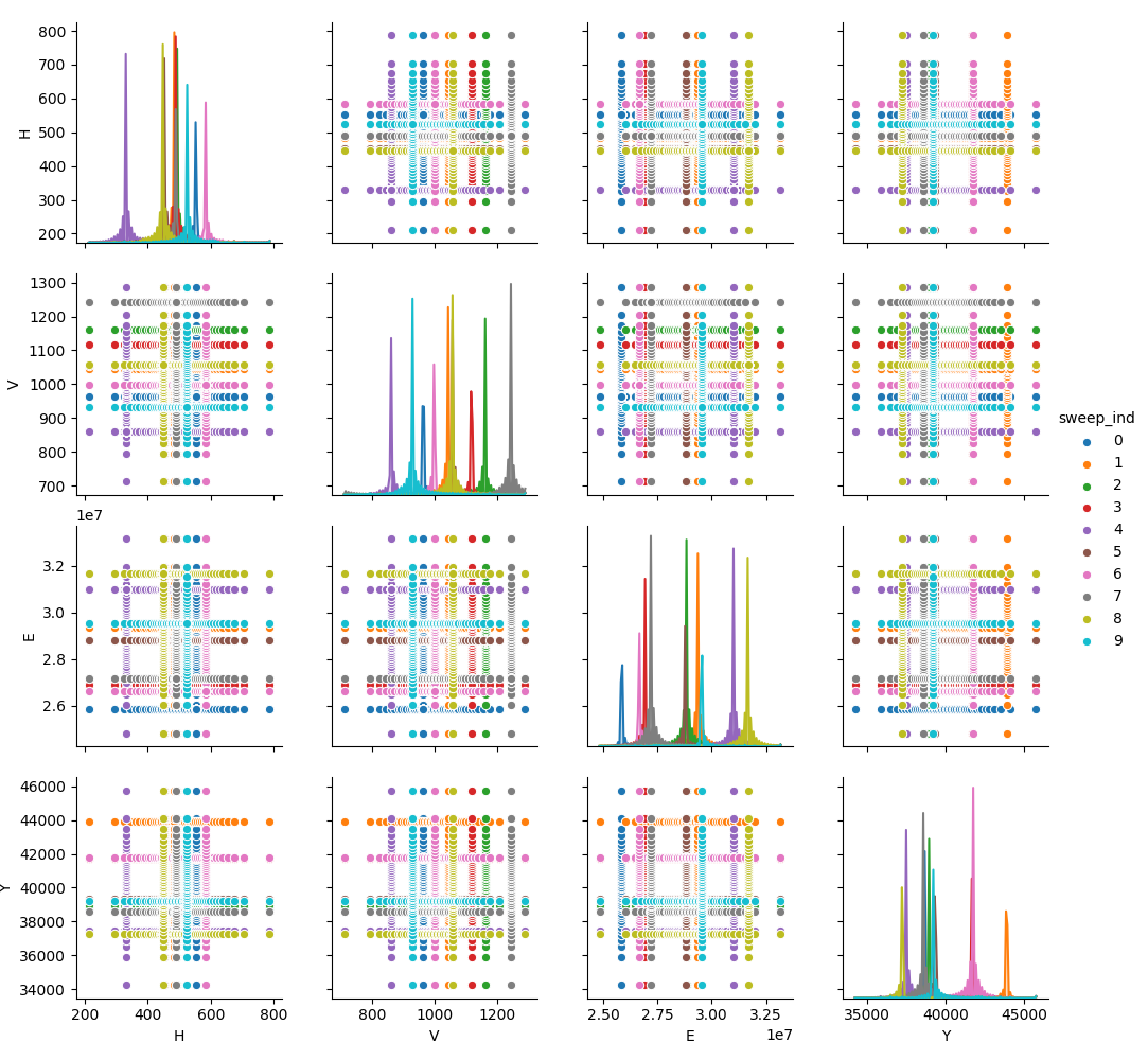../_images/ex_beam_sinews_doe.png beam sinew results

The “sinews” are sweeps across random variable space which start at random locations, and continue parallel to the variable axes. Evaluating these samples allows us to construct a sinew plot:

md_beam >> \
    gr.ev_sinews(n_density=50, n_sweeps=10, df_det="nom", skip=False) >> \
    gr.pt_auto()

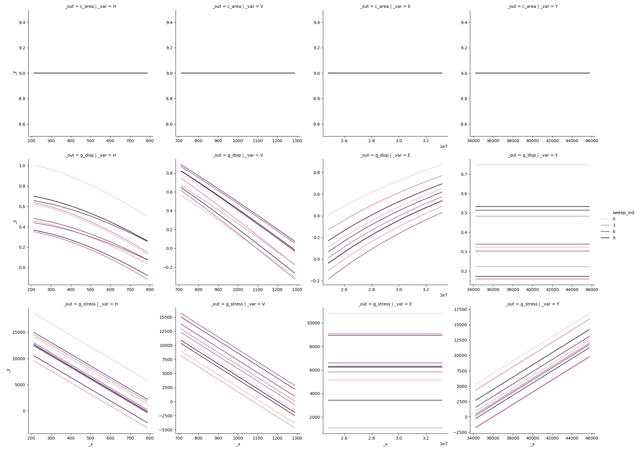../_images/ex_beam_sinews_res.png beam sinew results

Here we can see that inputs H,E tend to saturate in their effects on g_disp, while V is linear over its domain. This may explain the difference in contributed variance seen above via Sobol’ indices.

By providing tools to quickly perform different analyses, one can quickly get a sense of model behavior using py_grama.

Layers and Defaults¶

py_grama is built around layers and defaults. As much as is possible py_grama is designed to provide sensible defaults “out-of-the-box”. We saw the concept of layers above in the model building example. The following example shows defaults in action.

Example Defaults: `gr.eval_monte_carlo()`¶

Attempting to provide no arguments to gr.eval_monte_carlo() yields the following error:

df_res = md_beam >> gr.ev_monte_carlo()

...
ValueError: df_det must be DataFrame or 'nom'

One can sample over the random variables given their joint density, but this tells us nothing about how to treat the deterministic variables. The error message above tells us that we have to define the deterministic variable levels through df_det. To perform simple studies, we can explicitly limit attention to the nominal conditions.

df_res = md_beam >> gr.ev_monte_carlo(df_det="nom")
print(df_res.describe())

                H           V             E  ...  c_area    g_stress    g_disp
count    1.000000    1.000000  1.000000e+00  ...     1.0     1.00000  1.000000
mean   505.743982  906.946892  2.824652e+07  ...     9.0  9758.06826  0.438044
std           NaN         NaN           NaN  ...     NaN         NaN       NaN
min    505.743982  906.946892  2.824652e+07  ...     9.0  9758.06826  0.438044
25%    505.743982  906.946892  2.824652e+07  ...     9.0  9758.06826  0.438044
50%    505.743982  906.946892  2.824652e+07  ...     9.0  9758.06826  0.438044
75%    505.743982  906.946892  2.824652e+07  ...     9.0  9758.06826  0.438044
max    505.743982  906.946892  2.824652e+07  ...     9.0  9758.06826  0.438044

[8 rows x 9 columns]

By default gr.eval_monte_carlo() will draw a single sample; this leads to the NaN standard deviation (std) results. We can override this default behavior by providing the n keyword.

df_res = md_beam >> gr.ev_monte_carlo(df_det="nom", n=1e3)
print(df_res.describe())

eval_monte_carlo() is rounding n...
                 H            V             E  ...  c_area      g_stress       g_disp
count  1000.000000  1000.000000  1.000000e+03  ...  1000.0   1000.000000  1000.000000
mean    499.776481  1001.908814  2.899238e+07  ...     9.0   6589.731053     0.333387
std     100.878972   102.929434  1.523033e+06  ...     0.0   3807.292688     0.199576
min     168.466610   635.220875  2.427615e+07  ...     9.0  -5830.363269    -0.339594
25%     433.466349   933.698938  2.799035e+07  ...     9.0   3921.581411     0.200657
50%     500.201964  1002.514072  2.896188e+07  ...     9.0   6633.083925     0.339702
75%     569.159912  1065.489928  2.993924e+07  ...     9.0   9161.066426     0.465231
max     798.543698  1327.618914  3.378264e+07  ...     9.0  18682.531892     1.045742

[8 rows x 9 columns]

Formally 1e3 is a float, which is not a valid iteration count. The routine gr.eval_monte_carlo() informs us that it first rounds the given value before proceeding. Here we can see some variation in the inputs and outputs, though c_area is clearly unaffected by the randomness.

We can also provide an explicit DataFrame to the df_det argument. The gr.eval_monte_carlo() routine will automatically take an outer product of the deterministic settings with the random samples; this will lead to a multiplication in sample size of df_det.shape[0] * n. Since this can get quite large, we should reduce n before proceeding. We can also delay evaluation first with the skip keyword, and inspect the design first before evaluating it.

df_det = pd.DataFrame(dict(
    w=[3] * 10,
    t=[2.5 + i/10 for i in range(10)]
))

df_design = md_beam >> gr.ev_monte_carlo(df_det=df_det, n=1e2, skip=True)
print(df_design.describe())

eval_monte_carlo() is rounding n...
                 H            V             E             Y       w            t
count  1000.000000  1000.000000  1.000000e+03   1000.000000  1000.0  1000.000000
mean    485.021539   989.376268  2.890355e+07  40135.172902     3.0     2.950000
std     112.546373    92.381768  1.462286e+06   2135.788506     0.0     0.287372
min     137.606474   764.764234  2.586955e+07  33320.789307     3.0     2.500000
25%     411.652958   927.448139  2.763002e+07  39104.255172     3.0     2.700000
50%     490.765903  1002.513232  2.903287e+07  40121.853496     3.0     2.950000
75%     561.317283  1046.038620  2.994359e+07  41279.345157     3.0     3.200000
max     726.351812  1239.473097  3.176696e+07  45753.627265     3.0     3.400000

If we are happy with the design (possibly after visual inspection), we can pass the input DataFrame to the straight evaluation routine

df_res = md_beam >> gr.ev_df(df=df_design)
print(df_res.describe())

                 H            V             E  ...       c_area      g_stress       g_
disp
count  1000.000000  1000.000000  1.000000e+03  ...  1000.000000   1000.000000  1000.00
0000
mean    510.457048  1003.972079  2.887534e+07  ...     8.850000   4555.508097     0.12
0805
std     105.566743    91.443354  1.486829e+06  ...     0.862116   7027.137049     0.59
9538
min     269.102628   830.234813  2.553299e+07  ...     7.500000 -18370.732185    -1.84
8058
25%     437.342719   939.490354  2.794973e+07  ...     8.100000   -385.620306    -0.29
7274
50%     515.387982   995.468715  2.868415e+07  ...     8.850000   5347.337598     0.23
2133
75%     584.899669  1054.815972  2.982724e+07  ...     9.600000   9824.615141     0.60
9096
max     775.221819  1257.095025  3.369872e+07  ...    10.200000  21238.954122     1.23
6387

[8 rows x 9 columns]

Functional Programming (Pipes)¶

Functional programming touches both the practical and conceptual aspects of the language. py_grama provides tools to use functional programming patterns. Short-stem versions of py_grama functions are pipe-enabled, meaning they can be used in functional programming form with the pipe operator >>. These pipe-enabled functions are simply aliases for the base functions, as demonstrated below:

df_base = gr.eval_nominal(md_beam, df_det="nom")
df_functional = md_beam >> gr.ev_nominal(df_det="nom")

df_base.equals(df_functional)

True

Functional patterns enable chaining multiple commands, as demonstrated in the following Sobol’ index analysis. In nested form using base functions, this would be:

df_sobol = gr.tran_sobol(gr.eval_hybrid(md_beam, n=1e3, df_det="nom", seed=101))

From the code above, it is difficult to see that we first consider md_beam, perform a hybrid-point evaluation, then use those data to estimate Sobol’ indices. With more chained functions, this only becomes more difficult. One could make the code significantly more readable by introducing intermediate variables:

df_samples = gr.eval_hybrid(md_beam, n=1e3, df_det="nom", seed=101)
df_sobol = gr.tran_sobol(df_samples)

Conceptually, using pipe-enabled functions allows one to skip assigning intermediate variables, and instead pass results along to the next function. The pipe operator >> inserts the results of one function as the first argument of the next function. A pipe-enabled version of the code above would be:

df_sobol = \
    md_beam >> \
    gr.ev_hybrid(n=1e3, df_det="nom", seed=101) >> \
    gr.tf_sobol()

References¶

I.M. Sobol’, “Sensitivity Estimates for Nonlinear Mathematical Models” (1999) MMCE, Vol 1.