Random Variable Modeling¶

Random variable modeling is a huge topic, but there are some key ideas that are important to know. This short chapter is a brief introduction to random variable modeling.

import grama as gr
DF = gr.Intention()

Random Variables in Grama¶

Random variables in grama are defined as part of a model. For instance, the following syntax defines a joint distribution for two inputs x and y.

(
    gr.Model("An example")
    # ... Function definitions
    >> gr.cp_marginals(
        x=gr.marg_mom("norm", mean=0, sd=1),
        y=gr.marg_mom("lognorm", mean=0, sd=1, floc=0),
    )
    >> gr.cp_copula_gaussian(
        df_corr=gr.df_make(var1="x", var2="y", corr=0.5)
    )
)

Grama defines joint distributions in terms of marginals and a copula. This definition is justified by Skylar’s Theorem, which states that an arbitrary joint distribution can be expressed in terms of its marginals and a copula. Practically, this modeling approach decomposes random variable modeling into two stages: Modeling the individual uncertainties with marginals, then modeling their dependency with a copula.

Running Example¶

As a running example, we will study the built-in die cast aluminum dataset.

from grama.data import df_shewhart

Marginals¶

Marginal distributions provide a quantitative description of uncertainty for a single quantity. Perhaps the most important factor in modeling a marginal is the shape of the distribution used to describe that quantity; there are often multiple competing distribution shapes that we could pick to fit the same dataset. For instance, the following code fits three different shapes to the tensile_strength in the example dataset.

mg_ts_norm = gr.marg_named(
    df_shewhart.tensile_strength,
    "norm", # Normal distribution
)

mg_ts_lognorm = gr.marg_named(
    df_shewhart.tensile_strength,
    "lognorm", # Lognormal distribution
    floc=0, # 2-parameter lognormal
)

mg_ts_gengamma = gr.marg_named(
    df_shewhart.tensile_strength,
    "gengamma", # Generalized gamma distribution
    floc=0, # 3-parameter generalized gamma
)

Visualizing the distributions gives three fairly plausible fits to the data:

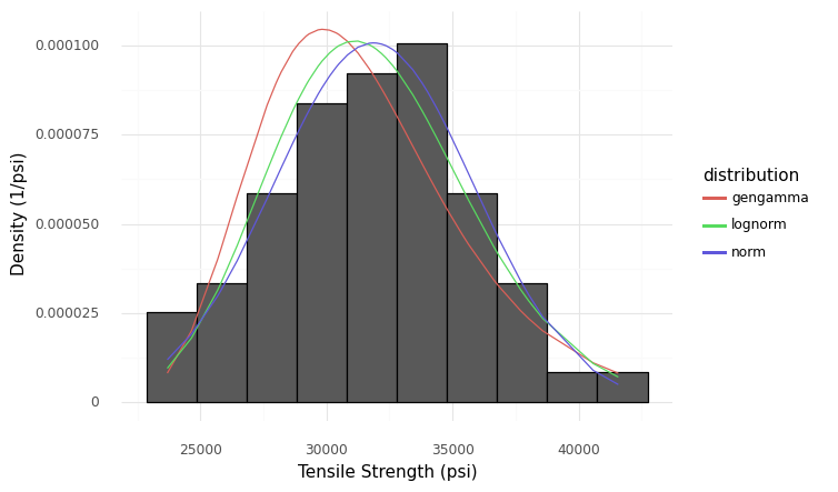../_images/shewhart-tys.png Comparison of three fitted distributions with a histogram of the tensile strength data

A more sensitive way to make this comparison is with a QQ plot.

(
    df_shewhart
    >> gr.tf_mutate(
        q_norm=gr.qqvals(DF.tensile_strength, marg=mg_ts_norm),
        q_lognorm=gr.qqvals(DF.tensile_strength, marg=mg_ts_lognorm),
        q_gengamma=gr.qqvals(DF.tensile_strength, marg=mg_ts_gengamma),
    )
    >> gr.tf_pivot_longer(
        columns=["q_norm", "q_lognorm", "q_gengamma"],
        names_to=[".value", "distribution"],
        names_sep="_",
    )

    >> gr.ggplot(gr.aes("q", "tensile_strength"))
    + gr.geom_abline(intercept=0, slope=1, linetype="dashed")
    + gr.geom_point(gr.aes(color="distribution"))
    + gr.theme_minimal()
    + gr.theme(plot_background=gr.element_rect(color="white", fill="white"))
    + gr.labs(x="Reference Quantile", y="Observed Quantile")
)

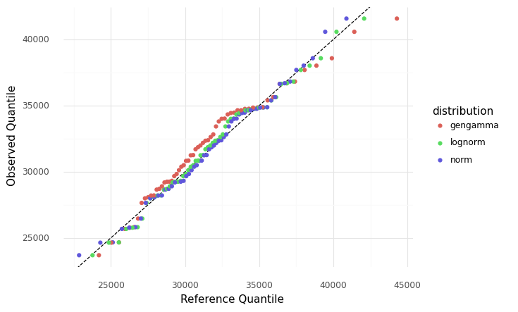../_images/shewhart-qq.png Comparison of three fitted distributions with a qq plot

This comparison reveals that the gamma distribution is shifted in its center, while the normal and lognormal fits are both fairly plausible.

Dependency¶

Marginals alone do not define a random variable. Dependency describes how values from different variables are related. Independent random variables are specified with an independence copula with gr.cp_copula_independence(). This is a common assumption, but it is frequently violated in practice.

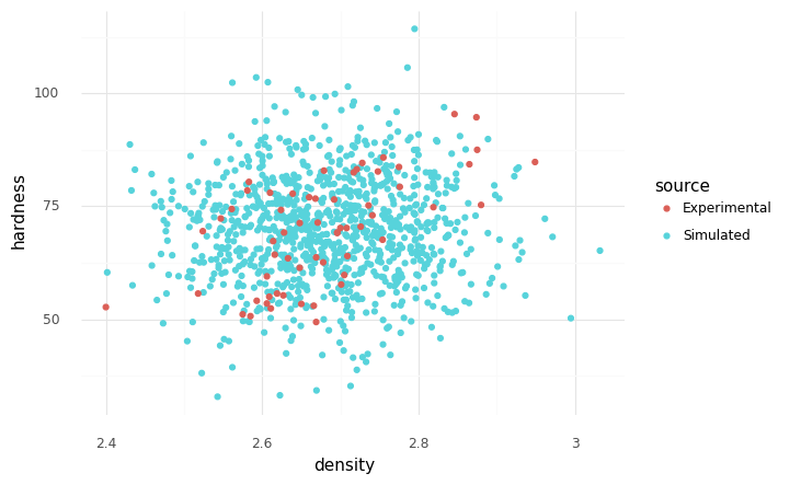../_images/shewhart-biv-indep.png Experimental and simulated observations, independent marginals

A simple way to represent dependency is with a gaussian copula, accessed with gr.cp_copula_gaussian().

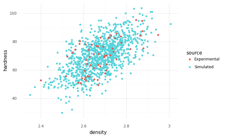../_images/shewhart-biv-gauss.png Experimental and simulated observations, gaussian copula

Note that it is critically important to state your assumptions when modeling random variables! You may have been sent to this page by an error message: That’s because grama requires you to make your assumptions about dependency explicit.